Dem Debate 1: Topic modeling
The second Democratic debate is almost here, so I wanted to follow up the sentiment analysis I performed on the first debate by looking at the topics that were talked about across the two nights.
In natural language processing, a topic model is a statistical model that can be used to infer the underlying meanings (i.e. topics) of utterances based on the words being used. In this post, I use Latent Dirichlet Allocation (LDA) from the topicmodels package to infer what each speech by the candidates is about. The model assumes:
Every speech is about a mixture of topics. For example, in a reply to a question by a moderator, a candidate might be speaking about the economy, or about the economy and climate change, etc. In contrast to other classification methods that try to identify only a single underlying category, LDA assigns probabilities to each topic, indicating the probability that a speech is about that topic.
Each topic of interest is spoken about using a reliable collection of words. For example, when speaking about a topic like healthcare, a candidate may use words like “insurance” and “medicare”. If we assume that an underlying topic generates certain words, each topic can be described as a collection of frequently co-occurring words.
Identifying topics
Determining the number of topics (k) that are talked about within a corpus (i.e. all speeches during the two nights of the first Democratic debate) is a tricky endeavour. There are various approaches to determining the optimal k (e.g., Griffiths & Steyvers, 2004; Arun et al., 2010), but these methods do not always converge. A more practical issue is that the optimal k computed via such methods may not be semantically meaningful.
For this post, I went with k = 4, because it led to semantically interpretable topics.1 The following figure displays the four topics the model identified in the transcripts of the first Democratic debate. Within each topic, the figure plots the beta weights of the top eight terms.2 Beta represents the probability of a term being generated by that topic. I believe the terms in each topic make the labels pretty self-explanatory.
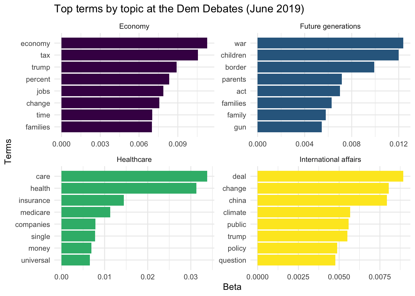
While the four topics – Economy, Future generations, Healthcare, and International affairs – are certainly not exhaustive, I believe they can be useful as broad categories for looking at patterns in what the debates were about.
Topics over time
After identifying the topics of interest, we can look at the inferences the model makes about each speech. For example, when Pete Buttigieg speaks at a particular juncture, what topic does the model infer as being the most probable? In the following figures, I display each topic’s gamma values for every speech (separately for the first and second nights of the debate). Gamma represents the probability of a speech being about a particular topic (gammas for all four topics sum to 1).
The speeches are arranged chronologically, painting a picture of how the topics being discussed changed over the course of each debate. In the first row, I have visualized the gamma values for each speech using bars, to illustrate the most salient topics at each point in time (note the changes in color). In the second row, I visualized the gamma values using points, and included trend lines to show how the the salience of each topic changed over time.
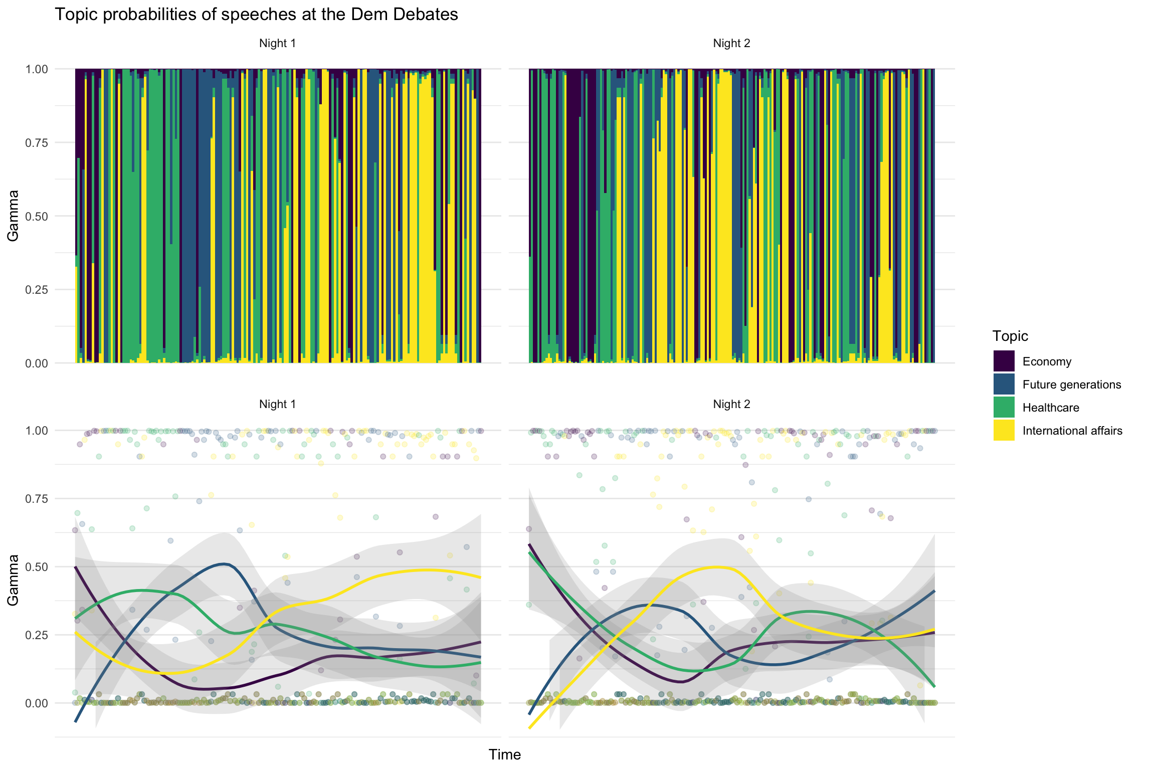
From these plots, it’s clear that on both nights, candidates started by talking about the economy (and to a lesser extent, healthcare). Around the quarter-mark, candidates started talking about issues faced by future generations (gun control, climate change, etc.). There were also differences; on the first night, candidates shifted to talking about international affairs towards the end of the debate, while on the second night this occured around the midpoint.
Topics by candidate
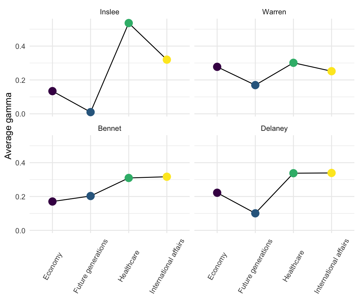
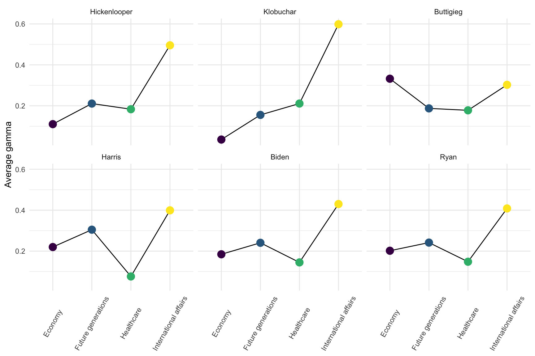
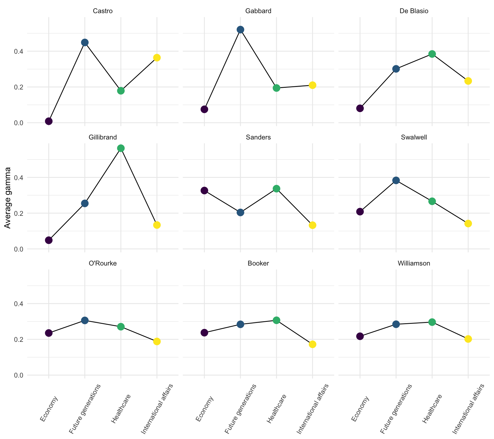
Finally, I wanted to see if candidates differed in the topics they tended to focus on in their speeches. To do this, I computed the average gamma within each topic for each candidate (higher average gammas indicate a candidate’s speeches were more likely to be about a particular topic). This results in candidate profiles of the relative importance of each topic.
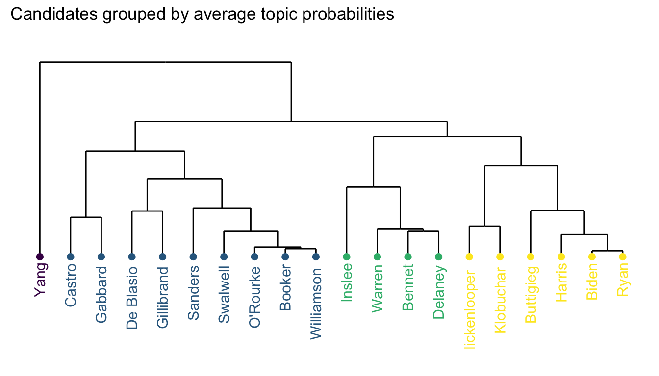
Before displaying these profiles, I wanted to categorize candidates based on their similarity to aid interpretation. To do this, I used hierarchical clustering (from the cluster package) to identify groups of candidates based on the pattern of their average gamma for the various topics. This clustering method identifies these groups based on the similarities between candidates, which I visualized in the following dendrogram. Based on the relative importance of each topic in their speeches, there are four groups of candidates.
Economy-plus candidate
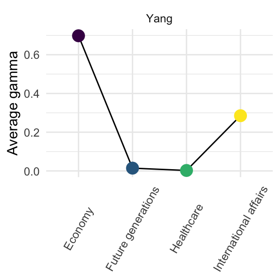
First comes Andrew Yang in a class of his own. He only made seven speeches, but focused very heavily on the economy relative to other topics.
Healthcare-now candidates
The following four candidates have topic distributions that favor healthcare over talking about issues facing future generations.
Worldly candidates
These six candidates seemed to focus just a bit more on international affairs than other topics.
Scattered candidates
It’s hard to succintly describe the patterns of the remaining nine candidates. I couldn’t help notice that Cory Booker’s topic distribution is eerily similar to Marianne Williamson. They might want to do more to differentiate themselves.
Conclusion
Natural language processing is complex. While using a model to infer topics from speech helps in understanding broad patterns and trends, no list of topics will fully capture the topics that were actually being spoken about. While the LDA model used here assumes that each topic is identifiable based on particular terms, different candidates may use terms in different ways.
Furthermore, when considering the topics different candidates tend to focus on, it’s worth noting that the topics they address are influenced by moderators and the speeches of other candidates that came before. While the plots above reveal the topics each candidate focused on during the last debate, this does not necessarily correspond to the importance the candidate places on that topic.
Despite these limitations, I believe that such analyses are useful for gaining a general picture of the topics candidates were focusing on in their speeches.
Evelyn Yarzebinski found this approach lacking, so I used the
ldatuningpackage to evaluate the optimal k. However, this led to an optimal k of 9 or 10, resulting in topics with terms that were hard to meaningfully discern. I didn’t want to sacrifice interpretability, hence my decision to stick with k = 4.↩I excluded stopwords (“the”, “and”, “a”…) and non-diagnostic words that were associated with multiple topics (“president”, “america”, “country”, “people”, and “united states”).↩